Recently the Ethereum Foundation announced a Proximity Prize for the resolution of the proximity gaps conjecture for Reed—Solomon Codes. This immediately sparked interest in the community, and in the past days several new results have appeared that give strong results in the direction of the conjecture or counterexamples in specific domains of the parameters:

• On the Distribution of the Distances of Random Words by Benjamin E. Diamond and Angus Gruen, cryptoeprint:2025/2010
• On Reed–Solomon Proximity Gaps Conjectures by Elizabeth Crites and Alistair Stewart, cryptoeprint:2025/2046
• Optimal Proximity Gaps for Subspace-Design Codes and (Random) Reed-Solomon Codes by Rohan Goyal and Venkatesan Guruswami, ECCC, Report No. 166 (2025)
• On Proximity Gaps for Reed-Solomon Codes, by Eli Ben-Sasson, Dan Carmon, Ulrich Haböck, Swastik Kopparty and Shubhangi Saraf, ECCC, Report No. 169 (2025)
• Deterministic list decoding of Reed-Solomon codes, by Soham Chatterjee, Prahladh Harsha and Mrinal Kumar, ECCC, Report No. 170 (2025)
• All Polynomial Generators Preserve Distance with Mutual Correlated Agreement, by Sarah Bordage, Alessandro Chiesa, Ziyi Guan, Ignacio Manzur, cryptoeprint:2025/2051

All of them also contain results, which are interesting in their own sake.

The aim of these notes is to give an accessible introduction to the Proximity Gaps Conjecture and the related notion of correlated agreement. In a follow-up note we will explain the results obtained in the above preprints, their implications for the soundness of various protocols that depend on them and the security of zkVM’s that depend on these protocols.

We will give a layered exposition, starting with a basic introduction and analogies and try to dive deeper as we progress.

The gap

Let’s start with the notion of the “gap”. This reflects the phenomenon of having a strong dichotomy. Given a set of elements, we want to say that either only very few of the elements of the set, or all of them have a certain property (we will specify what “few” means later). For example, it should not be the case that say half of them have the property and the other half does not.

We will say that a collection of sets displays a gap if every set in the collection has this dichotomy (only very few or all). It should be stressed that this is a property of the collection of sets, which makes things a bit more complicated.

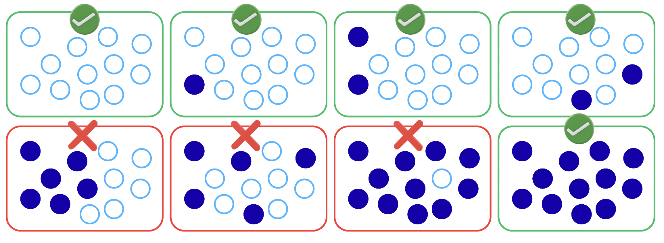
As an example consider a line L in the plane. For a point in the plane, let the property under consideration be “the point is on the line”. Now a set consists of several points. If you consider the collection of lines in the plane (each set in the collection is the set of points on a line), you will see a gap.

Given a set (a line), either very few of its points are on the line L in the plane (0 or 1), or, as soon as 2 points of the line are on L, the lines will coincide and all points will be on the line. These three scenarios are shown in the first three figures below. There is no line that contains 3 or more points of L without every point being on the line.

If on the other hand, your collection consists of all sets of points in the plane, you will definitely observe no gap. Arbitrary sets may have half of the elements on the line and the other half not on the line. This situation is shown in the bottom right figure above.

The proximity

For ZK proof systems like STARKs, Ligero, Aurora and Fractal, a relevant property is “being a polynomial of a certain degree”. More precisely, we have the following setup: given a finite field \mathbb{F}_q and a fixed domain D \subseteq \mathbb{F}_q of cardinality n, we consider functions f : D \to \mathbb{F}_q. We fix a scalar k and ask whether f is a polynomial of degree less than k.

For two functions f, f' : D \to \mathbb{F}_q we define their (Hamming) distance d(f,f') to be the number of inputs in D at which they differ. Given a non-negative integer bound d, we want to know whether it is true that for some polynomial p \in \mathbb{F}_q[x] of degree less than k, we have d(f,p) < d, i.e., the value of f differs from the values of p less than d locations in D. Rather than the absolute distance d it is customary to consider the relative parameter \delta = d/n, i.e., the fraction of the domain D at which the functions differ. This proximity property under consideration is the proximity to polynomials of degree less than k.

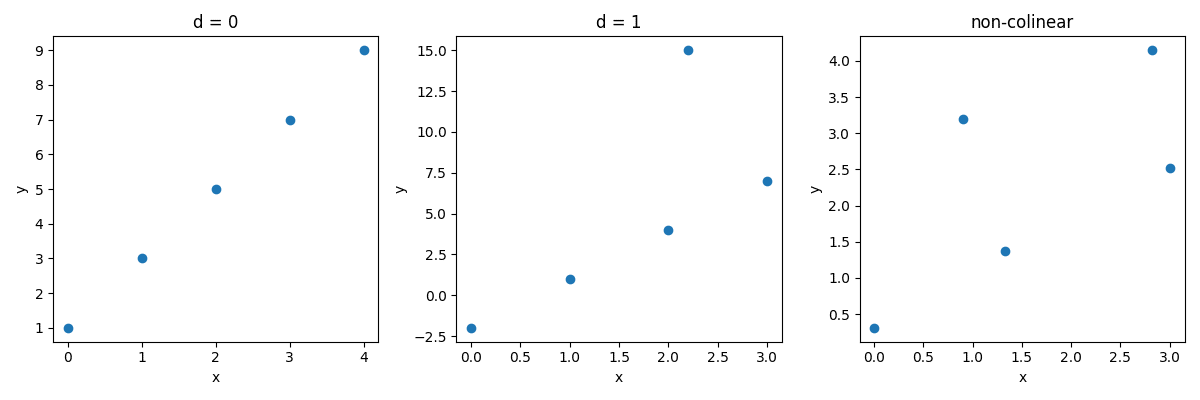
For example, if k=1 then we are asking: what fraction of the points lie along some line? In the below example, the first set of points has Hamming distance 0 from the set of degree-1 polynomials (all points in the set lie on a line), the second has Hamming distance 1 from the set of degree-1 polynomials (a line goes through all but one of the points), and the third has Hamming distance 3 from the set of degree-1 polynomials (every line misses at least 3 of the points in the set).

Having specified what the property of interest is, the next question is what the sets for which we hope to have the gap phenomenon. It does depend on the application in mind and the Proximity Gap Theorem comes in many guises.

Proximity gaps for affine spaces

As a first case consider the following: for a pair of functions f_1 and f_2 consider the set consisting of functions of the form f_1 + \lambda \cdot f_2 for \lambda \in \mathbb{F}_q. Note that this corresponds to the “line” through f_1 in the direction of f_2.

The proximity gap for affine spaces requires that for each set of functions as above, either only a few of them are close to a polynomial of degree less than k, or all of them are so. Depending on the precise choice of definition for closeness (proximity) this is either a beautiful theorem due to Ben-Sasson, Carmon, Ishai, Kopparty, or the famous proximity gaps conjecture.

Batching

Interesting as it is, what is its use? Here a first application: suppose you have a procedure at hand that allows you to prove that a given function is close to a polynomial of degree less than k. You claim that two functions f_1 and f_2 have this property. You could go ahead and apply your procedure to both of them one after the other. Alternatively you ask the person you want to convince to provide you with a random linear combination f_1 + \lambda \cdot f_2, i.e., to provide you with a random \lambda \in \mathbb{F}_q and do the proof for the random linear combination.

Now by the Proximity Gap Theorem, either all linear combinations are close, or only a few. If one of f_1 and f_2 is not close, then by the gap almost none of the linear combinations can be close! The probability of the random choice being among the few close ones is small. Hence if the random combination is close to a polynomial of degree less than k, then (with high probability) so are f_1 and f_2.

This is called batching, and leads to considerable savings and speed-ups in ZK proofs. Of course, one can take random linear combinations of more than two functions and utilize a generalization for the proximity gap theorem stated above.

By now, you should have a good sense of the core idea behind the Proximity Gap Theorem. In what follows, we’ll present the formal definition (with all the parameters), introduce a stronger version of the theorem, and show how it is used in the soundness proof of the FRI protocol. The discussion will become a bit more technical, but with the main idea in place, it should now be much easier to follow.

What is close, how much is few?

Now we need to precise what we mean by being “close” to a polynomial and there being only “few” close elements in the set. This will also help giving a more precise statement for the Proximity Gap Theorem / Conjecture.

First of all, if the distance to the polynomial we want to accept is too large, the statement will be vacuous, as if you allow yourself to move far enough, starting from any function you can reach a polynomial function of degree less than k. More precisely, given a function f on a domain D of size n, using Lagrange interpolation, you can find a polynomial p of degree less than k, which agrees with f on the first k points of the domain. So f and p can differ only in the remaining n-k points of the domain. Hence the distance of f to p is at most n-k. For every function there is a polynomial of degree < k at distance at most n-k. In other words, drawing balls of radius n-k around all polynomial functions of degree < k will cover the whole space of functions on D. So for distance d \ge n-k, the Proximity Gap Theorem will be vacuously true, as for any set, all elements will be n-k-close to a polynomial of degree < k.

If you work in relative parameters (dividing everything by n), letting \rho = k/n (this is called the rate), then for any proximity parameter \delta \ge 1 - \rho the theorem becomes trivially true.

So we are left with the case d \in (0, n-k) (or in relative parameters \delta \in (0, 1-\rho) ). The upper bound 1 - \rho is referred to as the capacity.

The Proximity Gap Theorem in its current form has been obtained in a sequence of great results and improvements by many people. Ben-Sasson, Carmon, Ishai, Kopparty and Saraf have shown the following result:

Up to the Unique Decoding Bound:

• The interval (0,\frac{n-k}{2}] (or (0, \frac{1-\rho}{2}) in relative parameters) is called the unique decoding regime. For a given function f there can be at most one polynomial of degree < k at distance at most \frac{n-k}{2}, as two such polynomials would differ in at most \frac{n-k}{2} + \frac{n-k}{2} = n-k points of the domain of size n and would hence agree at n - (n-k) = k points. But polynomials of degree < k that agree at k points have to be identical. This property can be exploited, there are various strong tools at hand (like the Berlekamp–Welch algorithm) that allow obtaining a proof for a Proximity Gap Theorem where few means a proportion less than \epsilon = n/q. For sets of elements of the form f_1 + \lambda \cdot f_2 this means either fewer than n elements are within d of a polynomial of degree less than k, or all of them are so.

Up to the Johnson Bound:

• For \delta in the interval (\frac{1-\rho}{2}, 1-\sqrt{\rho}), the minimal number of close elements grows quadratically with n, so for large enough n it is bounded by an expression of the form \epsilon = C \cdot n^2 (it was n in the region above). Here the constant C is allowed to depend on \delta and \rho.

The Proximity Gap Conjecture states that these bounds should be extendable until the capacity (so including the interval [1-\sqrt{\rho}, 1-\rho)) where the minimal number of close elements needed to conclude that all elements are close to a polynomial of degree < k should grow at most polynomially in n. This would mean that for all distances up to capacity, we have the dichotomy of either having few (bounded by a polynomial in n) close elements, or all.

Correlated agreement

How does one go about proving such a result? The statement to be proven says that if sufficiently many (more than just a few) functions in the set are each close to a polynomial, then all of them will be close. The way the closeness of each of them is realized can a priori be quite chaotic. Each element in the set can coincidentally be close to one of the polynomials, with no structure and deeper reason for why this happens. A correlated agreement result is a way of saying this happens because of some underlying structure. Proving the existence of such a structure is much easier than showing that one is lucky and coincidentally all elements are near. So, one shows that having more than some threshold of elements close can only happen when this structure exists, and the structure in turn implies that all elements must be close.

To understand the structure consider two functions from the set, say A = f_1 + \lambda_1 \cdot f_2 and B = f_1 + \lambda_2 \cdot f_2, which are close to polynomials p_1 and p_2 (both of degree < k) respectively. Now any other element C = f_1 + \lambda_3 \cdot f_2 in the set can be expressed as a linear combination of A and B:

B - A = (\lambda_2 - \lambda_1) \cdot f_2. If \lambda_3 = \lambda_1 + c \cdot (\lambda_2 - \lambda_1), then C = A + c \cdot (B - A).

As A is close to p_1 and B is close to p_2, we would hence hope the linear combination
C = A + c \cdot (B - A) to be close to the corresponding linear combination of the polynomials p_1 + c \cdot (p_2 - p_1).

Things are unfortunately not that easy. A might differ from p_1 at a set of points S that is different than the set R on which B differs from p_2. Then for the respective linear combinations, the values at which they differ will in general be the union of these sets S \cup R. Hence we will lose on closeness.

Except, of course, in the case these sets coincide: S = R. In that case, the linear combination will differ at the same points (at most). So C is also close to a polynomial of the right degree. Moreover, as all elements in the set can be expressed as a linear combination of A and B, all are close.

In this case there is a rigid structure in how things are close. Two basis elements (everything can be written in terms of them) are close to polynomials in such a way that the points where they differ from the respective polynomials agree. So the points where they agree with the polynomials agree. Hence the name correlated agreement. We can replace A and B above by f_1 and f_2.

The way the proximity gap is usually proven is as follows: Consider the set \{\, f_1 + \lambda \cdot f_2 \mid \lambda \in \mathbb{F}_q \,\}. One shows that if more than a certain number of elements in this set are close to polynomials of degree < k (agree with polynomials on large enough parts of the domain), then there exist polynomials u_1 and u_2 of degree < k which agree with f_1 and f_2 on a large part of the domain.

This is called the Correlated Agreement Theorem and is stronger than (i.e., implies) the Proximity Gap Theorem.

Soundness of the FRI protocol

Let’s see the Correlated Agreement Theorem in action. Consider the FRI-protocol (Fast Reed–Solomon Interactive Oracle Proofs of Proximity). It allows a prover to show that a function on a given domain D is close to a polynomial of degree < k with high probability. The domain D of size n is chosen so that the squaring map on D is 2-to-1, i.e., the set of squares of elements of D forms a set D^2 of half the size n/2. We will describe one step of FRI. More generally, we will want to repeatedly apply this construction, so D will be chosen as the roots of unity of 2-power order.

Rather than convincing the verifier that a function f is close to a polynomial of degree < k, the verifier will provide some random element r. The prover will “fold” the function f to a function f' on D^2, which is a domain of half the size, and reduce the task to a polynomial of half the degree on a domain half the size.

The values of a polynomial p(x) on D can almost be expressed in terms of the values of another polynomial of half the degree on D^2. If p(x) had only terms of even degree, we could write it as: p(x) = e(x^2) for some polynomial e(x) of degree < k/2, and for any \alpha \in D we have: p(\alpha) = e(\alpha^2) with \alpha^2 \in D^2.

As p(x) may also have odd terms, each of which can be written as x \cdot (\text{an even term}), we write it as p(x) = e(x^2) + x \cdot o(x^2) with polynomials e(x) and o(x) of degree < k/2. Here the values of p(x) on D are almost uniquely determined by e(x) and o(x) on D^2, were it not for the factor x.

Folding the polynomial now consists of using the randomness r provided by the verifier to replace the factor x and obtain the polynomial: e(x^2) + r \cdot o(x^2) = p'(x^2) with p'(x) = e(x) + r \cdot o(x).

The idea in the soundness argument of FRI boils down to using the Correlated Agreement Theorem to show that in case f is far (differs in at least d values) from a polynomial of degree < k, then for all but a few values of the random value r the folded function will be far (differs in at least d/2 values) from a polynomial of degree < k/2 on a domain of half the size. The proof is easy by the Correlated Agreement Theorem.

For the functions e_f and o_f on D^2 as above, denote f'_r = e_f + r \cdot o_f. If f'_r is d/2-close to a polynomial of degree < k/2 for more than just a few values of r, then there exist polynomials u_e and u_o of degree < k/2 such that e_f and o_f agree with u_e and u_o respectively on a large common set of points (all of D^2 except a set E of size at most d/2).

So: e_f(\alpha^2) = u_e(\alpha^2) and o_f(\alpha^2) = u_o(\alpha^2) for \alpha^2 \in D^2 \setminus E.

Now for such values of \alpha^2 we have:

f(\alpha) = e_f(\alpha^2) + \alpha \cdot o_f(\alpha^2) = u_e(\alpha^2) + \alpha \cdot u_o(\alpha^2)

So the value of f will agree with the degree < k polynomial u_e(x^2) + x \cdot u_o(x^2).

This happens for all \alpha such that \alpha^2 \notin E. As E is a set of size d/2, there are at most d such values of \alpha. So f agrees with a polynomial of degree < k at all but at most d values in D.

In other words, if f is d-far from a polynomial of degree < k, then for all but a few values of r (so with high probability) the fold f'_r will be d/2-far from a polynomial of degree < k/2. Repeating the folding and working out precise probabilities results in the well-known FRI protocol and its soundness argument.

Conclusion

We hope to have been able to give you a feeling for the statement of the Proximity Gap Theorem / Conjecture and why it is important. In the next post we will review some of the recent breakthrough results in this direction and implications for the zk-space (in particular for zkVM’s).

Authors:
Alp Bassa, Head of Cryptography
Ben Sepanski, Chief Security Officer